Background: Why Consider Autoregressive Models for 3D Molecule Generation?

1) Rethinking from AlphaFold2 and AlphaFold3 — Physical Constraints vs. Model Expressiveness.

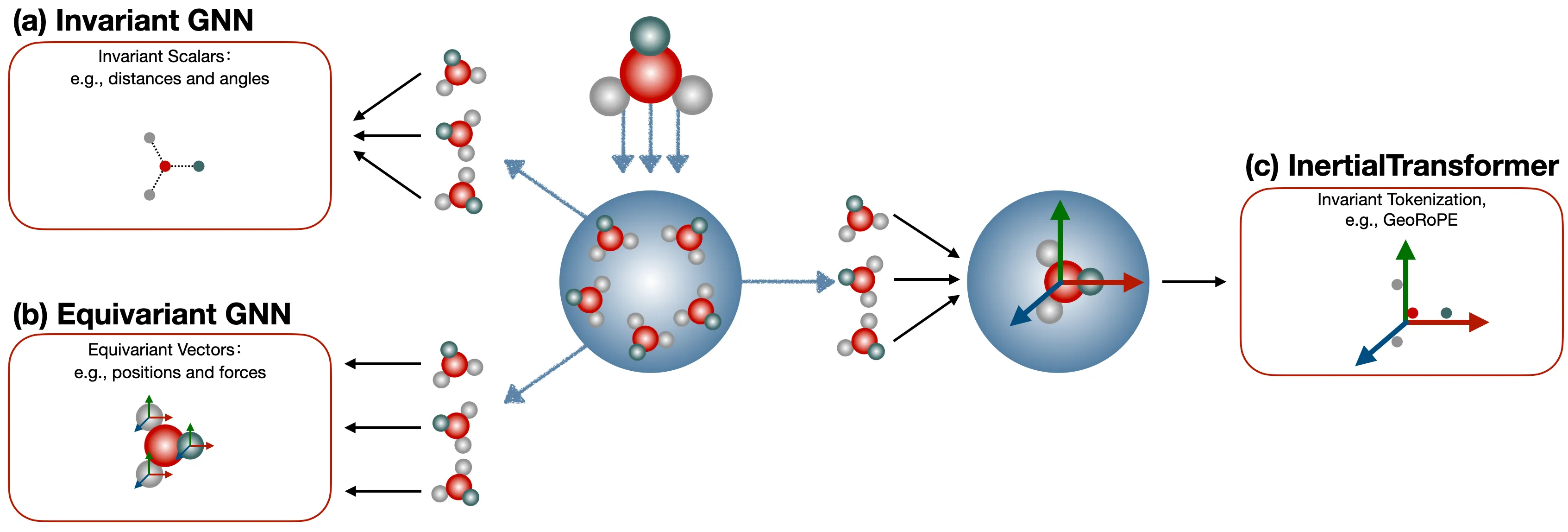
The core physical modeling in AlphaFold2 is Invariant Point Attention (IPA). It exploits the fact that the inner product between the bases of pairwise rigidity frames is invariant to rotation and translation. (If readers are interested, we can open a dedicated series to discuss this in depth.) This is essentially a form of constrained modeling — it sacrifices model expressiveness in exchange for 100% SE(3) equivariance. AlphaFold3, on the other hand, actually abandons perfect symmetry properties, instead using data augmentation to let the model learn to handle data in different poses as much as possible. This amounts to giving up perfect equivariance in order to unleash the model’s expressiveness.

So, thinking further along this line: is it possible to guarantee equivariance while simultaneously preserving maximum model expressiveness? The answer is yes. Through a data preprocessing approach — for instance, calibrating small molecules according to their inertial frame — we ensure that all small molecules use a unified global coordinate system, namely their own inertial frame. In this way, coordinate vectors that are inherently equivariant become invariant coordinate vectors. The remaining question is simply how to choose a highly expressive model to model these invariant vectors.

2) Why Choose When You Can Have Both — How to Make Transformers Perceive 3D Structure.

Following this direction, a very natural question arises: how can we use the most expressive models currently dominating CV, NLP, and AIGC — such as the Transformer — to perceive 3D molecular structures? Transformers consist of three main modules: token embedding, positional encoding, and self-attention. Our natural choice here is to design the Transformer’s positional encoding so that it can perceive 3D structures (there are many interesting reasons behind this, which we plan to explore further in Part 2).

In terms of specific implementation, we drew inspiration from Jianlin Su’s RoPE. However, if we simply apply RoPE to a 3-channel coordinate space, it essentially computes the L1 norm, or Manhattan distance. Here, we introduce Nyström estimation to compute the L2 norm, i.e., the Euclidean distance.

3) The Biggest Challenge from a GenAI Perspective — Simultaneous Generation of Continuous and Discrete Data.

This is a problem unique to many scientific domains. For example, in classical systems, the atom types of small molecules are discrete variables, while coordinates are continuous variables. How to generate both of them well simultaneously is a non-trivial matter. Currently, the mainstream generative paradigm in the 3D molecular domain is the Diffusion Model, such as EDM, which excel at continuous variables (coordinates) but are fundamentally designed for continuous spaces and require additional tricks when handling discrete variables (atom types). More critically, diffusion models rely on multi-step iterative denoising, leading to slow sampling, and they are inherently not good at handling variable-length sequences. Furthermore, existing 3D molecular diffusion models typically rely on SE(3)-equivariant GNN as backbones. Such specialized architectures have an inherent architectural barrier against the mainstream Transformer paradigm used across text and image modalities, making it difficult to integrate them into the unified framework of multimodal foundation models.

The Autoregressive (AR) model, in contrast, offers a complementary perspective. The core paradigm of AR models — Next Token Prediction — naturally supports variable-length generation and efficient decoding. However, classic AR models (such as GPT) only handle discrete tokens (picking a word from a vocabulary) and cannot directly regress continuous coordinates. If we forcibly discretize coordinates, precision is lost; if we forcibly use an L2 loss to directly regress coordinates, our experiments show that the model simply collapses. InertialAR’s solution is a very natural hierarchical strategy: first predict “what the next atom is” (discrete classification), then use Diffusion Loss to predict “where exactly it is” (continuous denoising), elegantly “nesting” the sequence generation capability of AR models with the continuous modeling capability of Diffusion.

SE(3) invariance guarantees, geometry-aware positional encoding, and discrete-continuous joint autoregressive generation — these constitute the three core puzzle pieces of InertialAR, corresponding to the three main methodological modules of the paper. Let us unfold them one by one below.

Deconstructing InertialAR: Aligning Molecules, Understanding Geometry, Generating Atom by Atom

Turning a Molecule into a Unique Sequence: Generation-Oriented Canonical Tokenization

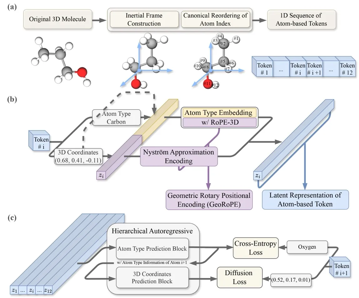
To do autoregressive generation, the first step is to convert a 3D molecule into a 1D sequence. The idea is straightforward: treat each atom as a token $a_{i} = (t_{i}, c_{i})$, where $t_{i}$ is the atom type and $c_{i}$ is the 3D coordinate. Arrange them in a certain order, and they can be predicted one by one just like a language model: $p(M) = \prod_{i=1}^{n} p(a_{i} \mid a_{< i})$.

But there is a key problem here: for the exact same molecule, rotating or translating it changes all the coordinates entirely; reordering the atoms produces a completely different sequence. If these “essentially identical” molecules are treated as different samples during training, the model cannot learn a consistent distribution. Therefore, we need to guarantee both SE(3) invariance and atom permutation invariance.

“Aligning” the molecule — Aligning to the Canonical Inertial Frame: Previously, to handle SE(3) invariance, models often had to design complex equivariant layers into the network architecture — like dancing in shackles, restricting the model’s potential. We instead choose to guarantee SE(3) invariance through data preprocessing, specifically borrowing the physics concept of the “inertial frame of reference”: every rigid body has its own principal axes of inertia. InertialAR first translates the molecule to its center of mass, then performs eigenvalue decomposition on the inertia tensor to obtain three orthogonal principal axes of inertia as the coordinate system. However, the three orthogonal axes still have ±1 directional ambiguities (yielding 4 possible right-handed coordinate systems). InertialAR uniquely determines the positive direction of the axes by selecting the farthest “anchor” atom. This way, no matter how the molecule was originally oriented in space, after this procedure it is “aligned” into the same canonical posture.

“Lining up” the atoms — Canonicalizing Atom Ordering: Even with the molecular orientation fixed, a molecule consisting of n atoms still has n! possible permutations. InertialAR uses RDKit’s canonical SMILES rules to deterministically sort atoms based on their chemical properties (atomic number, connectivity, ring membership, etc.), collapsing n! permutations into a single unique sequence.

At this point, each molecule corresponds to a unique token sequence, ready to be fed into the autoregressive model. But now that we have the sequence, how does the Transformer understand the 3D spatial relationships among these atom tokens? This brings us to the next module.

Making Transformers “Understand” 3D Geometry: GeoRoPE

Standard Transformers only recognize sequence position (the 1st token, the 2nd token, etc.) and are completely unaware of proximity relationships in 3D space — the fact that the i-th and j-th tokens attend to each other in the Attention mechanism does not mean the corresponding two atoms are closer or more related in geometric space. To make the Transformer truly “understand” molecular geometry, we chose to inject spatial information through positional encoding. But how exactly?

A very natural starting point is RoPE (Rotary Position Encoding). The reason Jianlin Su’s RoPE works so well is an elegant mathematical property: after transformation, the inner product of Query and Key depends only on their relative position, completely unaffected by absolute positions. InertialAR extends this idea from 1D sequences to 3D coordinate space — making Attention depend on the relative position vector $c_{i} - c_{j}$ between atoms, i.e., $(R_{c_{i}}q)^{\top}(R_{c_{j}}k) = q^{\top}R_{c_{j} - c_{i}}k$.

However, as pointed out in the background, simply applying RoPE to 3D coordinates essentially encodes along the x, y, and z axes independently, capturing something closer to the L1 norm (Manhattan distance), rather than the L2 norm (Euclidean distance) that we actually want. How do we bridge this gap? InertialAR introduces the Nyström method: through fixed anchor points, it performs a low-rank approximation of the RBF kernel matrix based on Euclidean distance, constructing feature vectors $z_{i}$ such that $z_{i}^{T}z_{j} \approx \text{RBF}(\| c_{i} - c_{j} \|)$, thereby injecting pairwise distance information into Attention in the form of a “vector dot product.” Thus, the final Attention Score takes the form:

$\text{Attn}(i,j) = q^{\top}R_{c_{j} - c_{i}}k + \text{RBF}(\| c_{i} - c_{j} \|)$

This achieves a complementary “parallel” design: the first term captures relative position, and the second term captures pairwise distance — the two working together.

There is a subtle but crucial engineering design point hidden here: why not just add the distance information directly as a bias to the Attention matrix? Because doing so would alter the standard Attention implementation, breaking compatibility with current mainstream LLM architectures. The essence of Nyström encoding is that it transforms pairwise distance computation into vector dot products, so geometric information can be processed just like ordinary token features, perfectly reusing standard matrix-multiplication Attention. This is also the key to InertialAR’s ability to scale up.

Letting AR Models Simultaneously Predict “What” and “Where”: Hierarchical AR with Diffusion Loss

With the sequence problem and geometry perception problem both solved, the final question returns to our discussion in the third point of the background: AR models are naturally good at discrete classification (picking a word), but cannot directly regress continuous coordinates. If you forcibly use an L2 loss to predict coordinates, the model simply collapses. So what do we do?

InertialAR’s approach is to split each step of “predicting the next atom” into two cascaded subtasks. First, it uses Cross-Entropy to predict the atom type (“Is the next one Carbon or Oxygen?”), then uses Diffusion Loss to predict its 3D coordinates (“Where exactly is it?”). Mathematically, this is a natural decomposition of conditional probability:

$p(a_{i+1} \mid h_{i}) = p(t_{i+1} \mid h_{i}) \cdot p(c_{i+1} \mid t_{i+1}, h_{i})$

Diffusion Loss vs. L2 Loss: Compared to stubbornly trying to regress an absolutely precise coordinate value, Diffusion Loss teaches the model to “denoise” — teaching the model how to step by step “wash out” the structure from noise. Ablation experiments also confirm that, within an autoregressive framework, using Diffusion to model continuous distributions is the necessary path to generating high-quality 3D structures, consistent with the findings of Kaiming He’s MAR.

Controllable Generation: Applying Classifier-Free Guidance to Both Branches Simultaneously

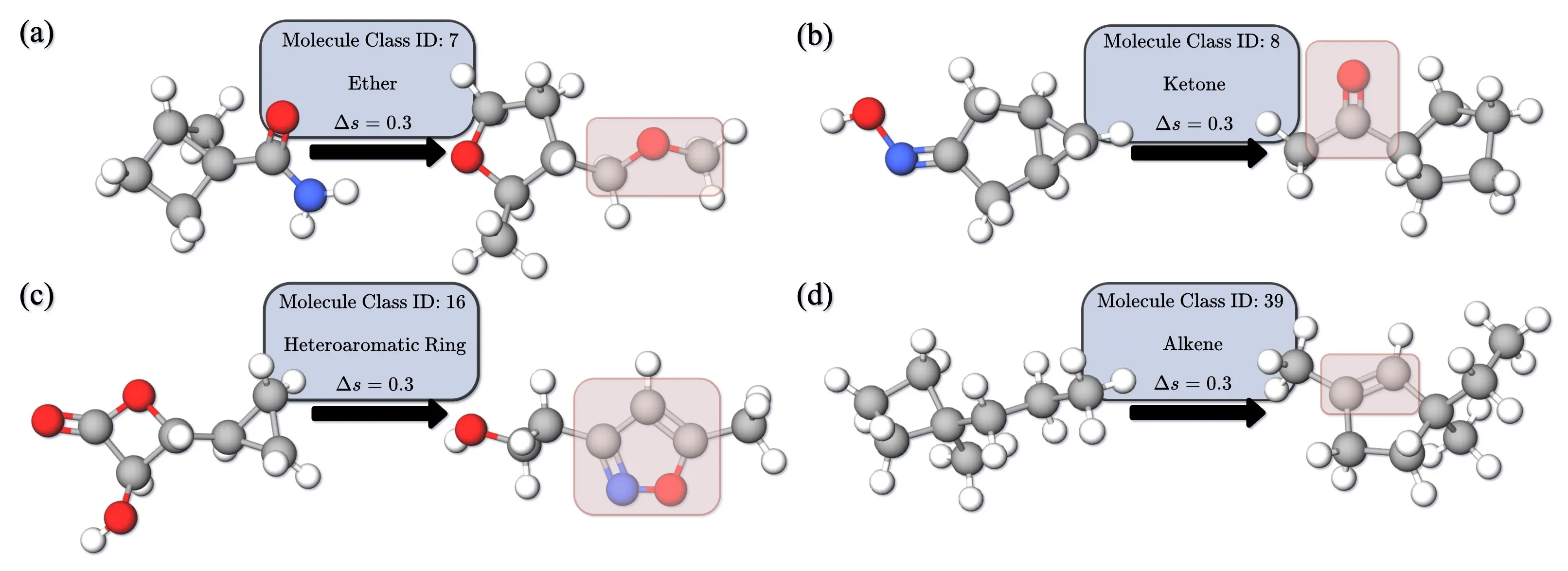
InertialAR also supports targeted 3D molecule generation conditioned on functional group categories. The specific approach introduces Classifier-Free Guidance (CFG): during training, a portion of category labels are randomly dropped, allowing the model to simultaneously learn both the conditional and unconditional distributions; during inference, the condition intensity is controlled via the guidance scale.

There is an interesting design choice here: many controllable generation methods only apply guidance on the continuous branch (coordinate denoising), but InertialAR also applies guidance on the logits of the type prediction. The reasoning is simple — if you only guide the coordinates without guiding the atom type selection, the generated atom type sequence itself may not match the target category, and no amount of coordinate adjustment will help. Adding CFG to both branches is necessary to simultaneously guarantee “chemical validity” and “conditional compliance.”

The paper also demonstrates an interesting extended application: by gradually increasing the guidance scale, an unreasonable molecule can be progressively “edited” into a reasonable structure satisfying the target category — similar to guided editing in the image domain.

Experimental Results

Unconditional Generation

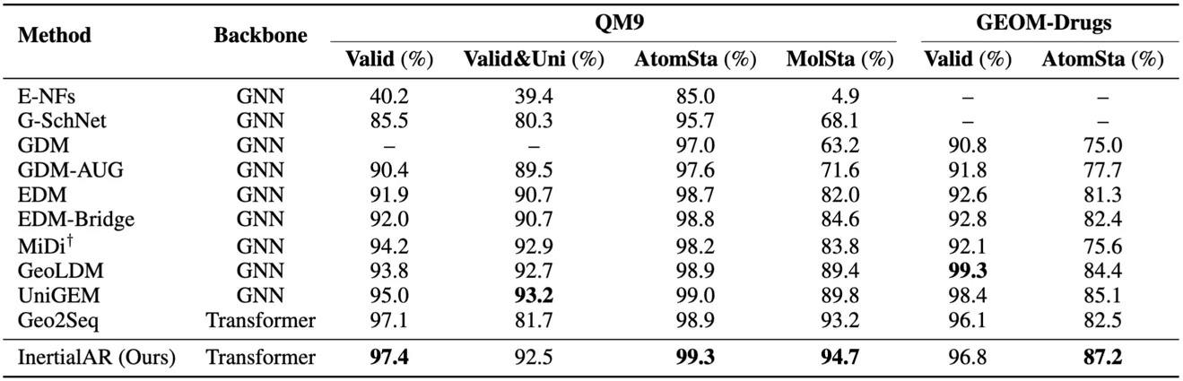
• QM9: InertialAR achieves the best performance on Valid (97.4%), AtomSta (99.3%), and MolSta (94.7%), surpassing all diffusion models and AR baselines.
• GEOM-Drugs: On the larger and more complex drug molecule dataset, InertialAR’s AtomSta (87.2%) is the highest among all methods, and Valid (96.8%) is second only to GeoLDM (99.3%).

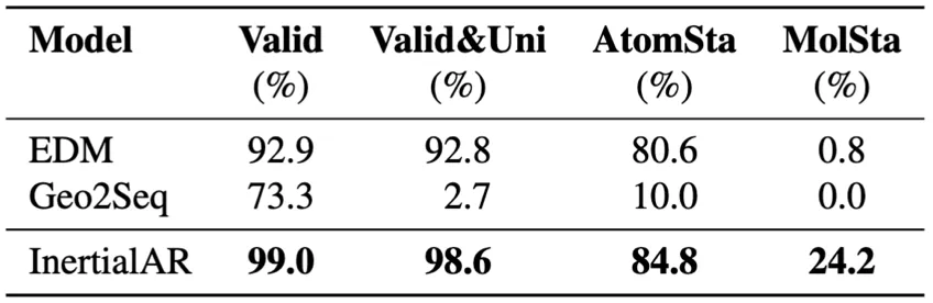
• B3LYP-1M (million-scale data): InertialAR achieves the best performance across all 4 metrics, with Valid 99.0%, Valid&Uni 98.6%, and MolSta 24.2%. This result strongly demonstrates InertialAR’s scaling capability — as data volume increases and chemical diversity grows, InertialAR not only shows no degradation but instead exhibits even stronger performance.

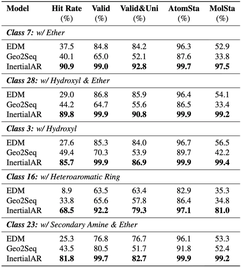
Controllable Generation (QM9, Class-conditional)

InertialAR achieves SOTA on all 5 evaluation metrics, with an average Hit Rate of 83.3%, significantly surpassing baselines. At the same time, with the help of Classifier-Free Guidance, InertialAR precisely meets the design requirements while maintaining the chemical validity of the molecules.

Conclusion and Outlook

Through three core modules — Generation-oriented Canonical Tokenization, the geometry-aware Attention mechanism (GeoRoPE), and the Hierarchical AR Paradigm — InertialAR successfully brings Transformer’s sequence modeling capability into the domain of 3D molecule generation. Across unconditional and controllable generation tasks combined, InertialAR achieves 8 SOTAs out of 10 unconditional generation metrics and sweeps all 5 controllable generation metrics.

Returning to the three questions raised in the background section, InertialAR provides a complete set of answers:

• Physical constraints vs. expressiveness? By canonicalizing the input (via the inertial frame), SE(3) invariance is guaranteed while the model’s expressiveness is fully liberated.
• How to make Transformers perceive 3D? Through GeoRoPE, injecting relative position and Euclidean distance information into the Attention mechanism.
• How to generate discrete and continuous data simultaneously? Through hierarchical AR + Diffusion Loss, achieving cascaded decoding.

The significance of this work goes beyond just a better-performing generative model; it points toward two exciting directions:

1. Extending to more complex scientific systems. InertialAR’s “canonicalization → tokenization → autoregressive generation” paradigm is not limited to small molecules. Protein structure modeling, periodic material design, and similar domains all face challenges involving SE(3) symmetry and variable-length structures — this methodology has natural potential for cross-domain transfer.

2. Unified multi-modal modeling. Since 3D molecular structures can be canonicalized into one-dimensional token sequences, they inherently possess the foundational conditions for joint modeling with text, images, and other modalities under a unified Transformer framework — this is precisely the key step needed for building multimodal foundation models in the scientific domain.

---

Cite Us:

@misc{li2025inertialarautoregressive3dmolecule,
  title={InertialAR: Autoregressive 3D Molecule Generation with Inertial Frames},
  author={Haorui Li and Weitao Du and Yuqiang Li and Hongyu Guo and Shengchao Liu},
  year={2025},
  eprint={2510.27497},
  archivePrefix={arXiv},
  primaryClass={cs.LG},
  url={https://arxiv.org/abs/2510.27497},
}